The goal of adaptive Markov Chain Monte Carlo is to develop more efficient samplers by adapting the Markov transition operator during sampling.

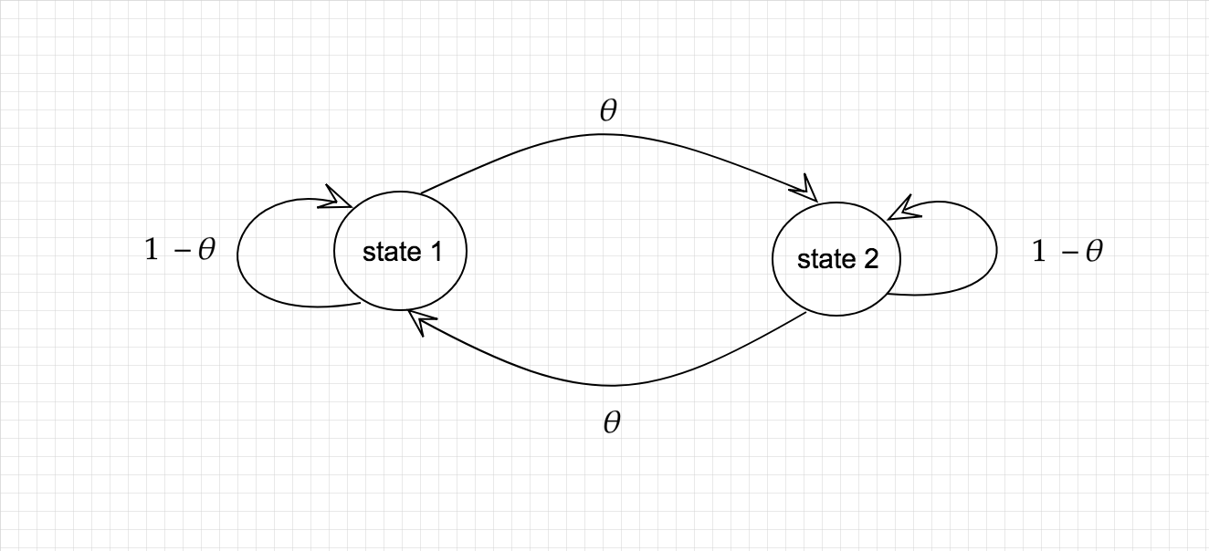
An easy mistake to make is to think that as long as during adaptation the Markov operator always has the correct stationary distribution then the overall sampler will be correct but this is not true. Here’s a simple intuitive example that shows that this is not correct. Imagine that we wish to sample from a Bernoulli distribution where each state has an equal probability of being sampled. We could doing this by simulating from the Markov chain shown in the picture below. The arrows represent possible transitions and their probabilities.

It’s clear by symmetry that if we start in state 1 and hop along the arrows according to the probabilities shown, that we’ll spend an equal amount of time in both states no matter what the value of $\theta$ is. So following this Markov chain would allow us to simulate from a fair coin and we could change the starting value of $\theta$ and have no affect.

What would happen however, if we started simulating this Markov chain and then changed the value of $\theta$. Well initially both states 1 and 2 would be equally likely by symmetry but when I change $\theta$, lets say made it bigger, then the state the chain is in when $\theta$ becomes bigger will now be less likely than the other state. Overall, our chain will no longer be simulating from a fair coin. This is despite the fact that if we first fixed $\theta$ to any value and then simulated with that fixed $\theta$, we’d always simulate a fair coin.

This shows that care must be taken when adapting transitions during MCMC. For most chains we can guarantee that adaptation wont break our sampler as long as the amount of adaptation tends to $0$ as the length of the chain tends to infinity. This criterion is known as “vanishing adaptation”. In general we should use adaptation with caution.